Regression Analysis
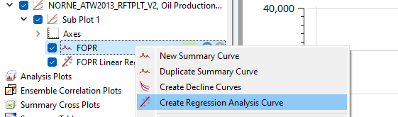
Create Regression Analysis
Regression analysis curves can be created from the right-click menu for a curve in the Plot Project Tree. In addition to single curves, regression anaysis is also supported on ensemble statistics curves and Cross Plot curves.
Regression Types
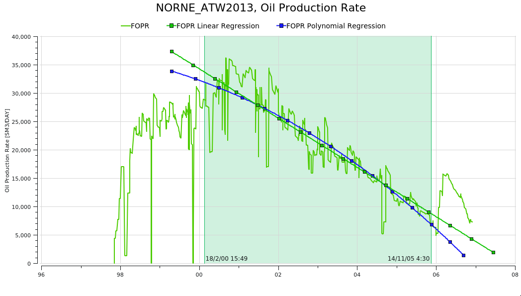
Linear Regression
The linear regression (i.e. straight line fit) is calculated by choosing the line that minimizes the sum of the squared differences between the observed dependent variable values and the values predicted by the linear equation. The straight line equation can be written as:
$$ y = a + bx $$
where:
- $y$ is the dependent variable,
- $x$ is the independent variable,
- $a$ is the intercept,
- $b$ is the slope.
Polynomial Regression
Polynomial regression is a form of linear regression where the relationship between the independent variable(s) and the dependent variable is modeled as an nth-degree polynomial. It allows for more complex relationships between the variables by introducing polynomial terms into the regression equation.
A polynomial in a single indeterminate x can always be written (or rewritten) in the form
$$ y = a_{n}x^n + a_{n-1}x^{n-1} + \dots + a_{2}x^{2}+a_{1}x+a_{0} $$
where:
- $a_0 , \ldots, a_n$ are constants that are called the coefficients of the polynomial,
- $x$ is the indeterminate.
- $n$ is the degree of the polynomial.
To determine the degree of the polynomial, one needs to consider the complexity of the relationship between the variables and the nature of the data. A higher degree polynomial can capture more intricate relationships but may also lead to overfitting if the model becomes too flexible.
Polynomial regression can be beneficial when the relationship between the variables is curvilinear or nonlinear. By introducing polynomial terms, it can capture the curvature in the data and provide a better fit compared to simple linear regression.
Power Fit Regression
The Power Fit regression is described by the following equation:
$$ y = ax^b $$
where:
- $y$ is the dependent variable,
- $x$ is the independent variable,
- $a$ is the coefficient,
- $b$ is the exponent.
In power fit regression, the goal is to estimate the values of $a$ and $b$ that best describe the relationship between the variables. This is done by minimizing the sum of the squared differences between the observed dependent variable values and the values predicted by the power-law equation.
Exponential Regression
Exponential regression is a type of nonlinear regression used to model relationships where the dependent variable changes exponentially with the independent variable. It is suitable when the data exhibits exponential growth or decay patterns.
The equation for exponential regression can be written as:
$$ y = ae^{bx} $$
where:
- $y$ is the dependent variable,
- $x$ is the independent variable,
- $a$ is the coefficient,
- $b$ is the rate of growth or decay,
- $e$ is the base of the natural logarithm (approximately 2.71828).
Exponential models are commonly used in biological applications, for example, for exponential growth of bacteria. Spotfire uses a nonlinear regression method for this calculation. This will result in better accuracy of the calculation compared to using linear regression on transformed values only.
Logarithmic Regression
The logarithmic fit calculates the least squares fit through points by using the following equation:
$$ y = a + b \ln( x ) $$
- $y$ is the dependent variable,
- $x$ is the independent variable,
- $a$ and $b$ are coefficients.