Well Log Plots
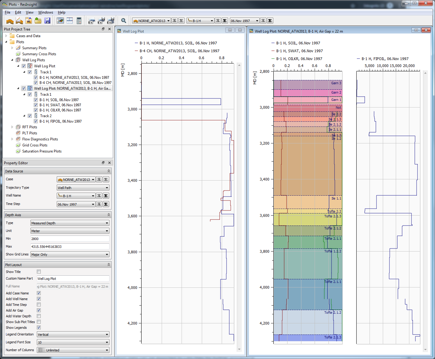
ResInsight can display well logs by extracting data from a simulation model along a well trajectory and from imported LAS-files. Extracted simulation data can be exported to LAS-files for further processing.
Well Log Plots
Well log plots can be created in several ways:
- Right-click a well path or a simulation well in the 3D-view and select New Well Log Extraction Curve.
A new plot with a single Track and Curve is created matching active case and selected Well trajectory. - Right-click Well Log Plots in the Plot Project Tree and select New Well Log Plot. A plot is created with one Track and Curve.
- Right-click
 Wells
in the Project Tree and select Import->Import Well Logs from file.
Wells
in the Project Tree and select Import->Import Well Logs from file.
Each Well Log Plot can contain several Tracks, and each Track can contain several Curves.
Tracks and Curves can be organized using drag and drop of their entries in the Plot Project Tree. Tracks can be moved from one plot to another and you can alter the order of tracks within a Well Log Plot by drag and drop. In addition, Curves can be moved from one Track to another. Furthermore, copy and paste of a Well Log Plot, Track, and Curve is possible by right-clicking their entry.
Measured Depth (MD), True Vertical Depth (TVD), True Vertical Depth RKB (TVDRKB) and Pseudo Length (PL)
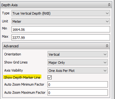
All Tracks in the same Well Log Plot always display the same depth range, and share the True Vertical Depth (TVD) or Measured Depth (MD) setting. In the property panel of the plot, the exact depth range can be adjusted along with the depth type setting (TVD/MD).
Simulation Wells however, is using a Pseudo Length instead of the real Measured Depth when the depth type is MD, as the MD information is not available in restart files. The Pseudo Length is a length along the coarsely interpolated visualization pipe, and serves only as a coarse estimation of an MD-like depth. Pseudo length is measured from the simulation-wells first connection-cell (well head connection) to the reservoir. This is very different from MD, which would start at RKB or at sea level.
Depth Unit
The depth unit can be set using the Depth unit option. Currently ResInsight supports Meter and Feet. The first curve added to a plot will set the plot unit based on the curve unit. Additional curves added to a plot will be converted to the plot unit if needed.
Depth Zoom and Pan
The visible depth range can be panned using the mouse wheel while the mouse pointer hovers over the plot. Pressing and holding CTRL while using the mouse wheel will allow you to zoom in or out depth-wise, towards the mouse position.
Depth Marker Line
If there are multiple tracks in the same plot, it can be useful to show a horizontal line across the plot based on the location of the mouse cursor. This can be activated from the Property Editor of a Well Log Plot.
Accessing Plot Data
Right-click a Well Log Plot and select Show Plot Data to show a window containing the plot data in ascii format. The content of this window is easy to copy and paste into Excel or other tools for further processing.
It is also possible to save the ascii data to a file by selecting a Well Log Plot in the Plot Project Tree and use the right-click command Export Plot Data to Text File.
Tracks
Tracks can be created by right-clicking a Well Log Plot and select New Track.
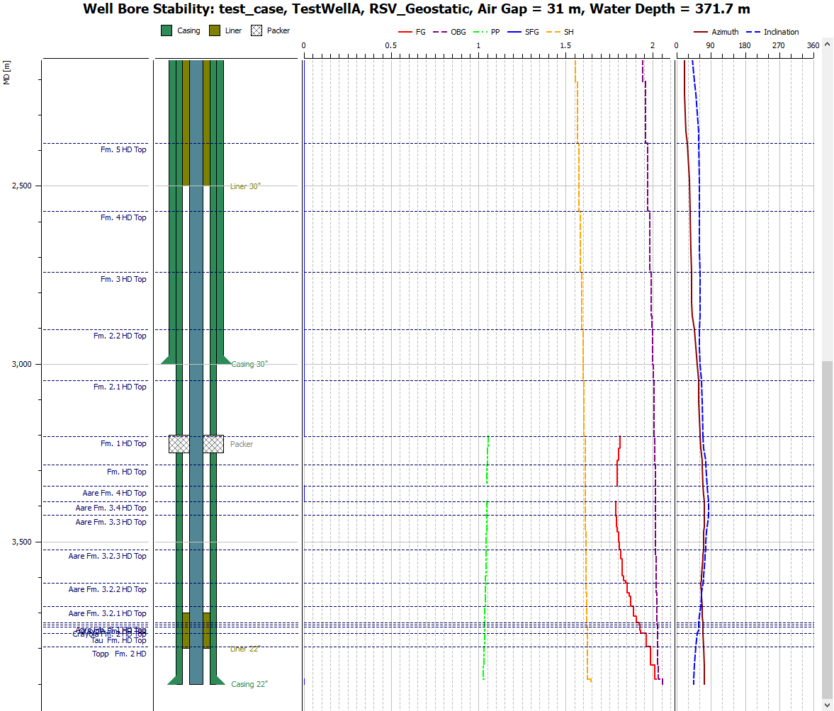
The settings of each Track is controlled by the Property Editor. The figure below shows settings for the middle Track shown in the figure at top of this page which is annotated by Formations in Category colors. For GeoMechanical models, adding formations will also indicate the sea level.
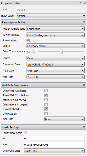
A track controls the x-axis range of the display which is set in the property panel. In addition to the range, logarithmic display is controlled by checking Logarithmic Scale, grid lines are controlled by the Show Grid Lines option.
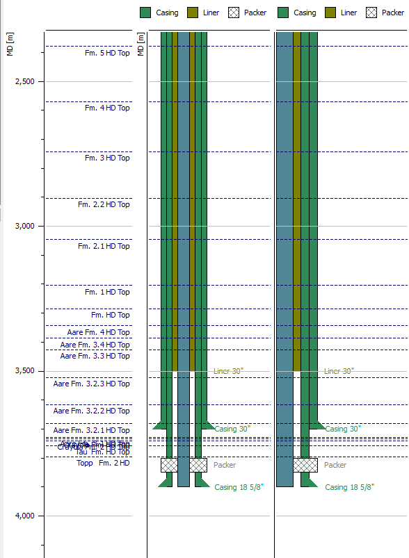
It is also possible to visualize Well Attributes such as casing and liners. The following images show some of the possibilities in which the first track shows cross sections of a well and the second track shows a radial view labeled with formations.
Curves
Curves can be created by right-clicking a Track in the Plot Project Tree or by the commands mentioned above. The two types of curves are Well Log Extraction Curves and Well Log LAS Curves.
Well Log Extraction Curves
Extraction curves acts as an artificial well log curves. Instead of probing the real well, a simulation model is probed instead.
The property panel for an eclipse model is shown below:
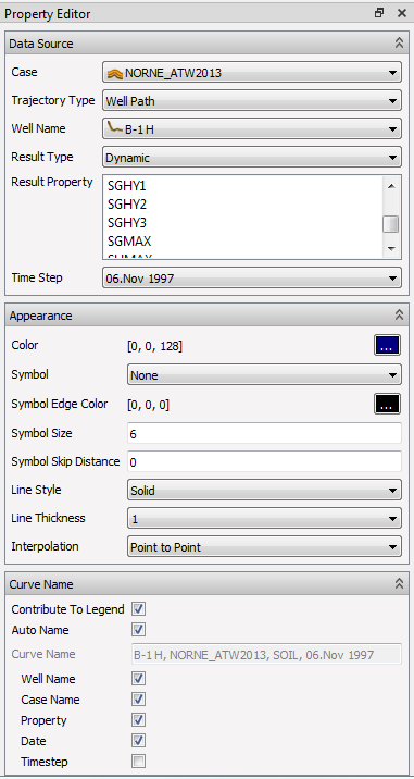
The first group of options controls all the input needed to setup curve data extraction. The selection of result value is somewhat different between geomechanical cases and Eclipse cases. Time step can be specified for dynamic properties.
Curve visual appearance and naming is controlled by the Appearance and Curve Name sections. The display name of a curve is normally generated automatically. Optionally, Auto Name can be switched off to use the options below to tailor curve name.
Note
Placing keyboard focus in the Time Step drop-down box allows you to use arrow keys or mouse wheel to quickly step through the timesteps while watching the changes in the curve.
Curve Extraction Calculation
This section describes how the values are extracted from the grid when creating a Well Log Extraction Curve.
Extraction curves are calculated by finding the intersections between a well trajectory and the cell-faces in a particular grid model. Usually there are two intersections at nearly the same spot; the one leaving the previous cell, and the one entering the next one. At each intersection point the measured depth along the trajectory is interpolated from the trajectory data. The result value is retrieved from the corresponding cell in different ways depending on the nature of the underlying result.
For Eclipse results the cell face value is used directly. This is normally the same as the corresponding cell value, but if a Directional combined results is used ( See Derived Results ), it will be that particular face’s value.
Abaqus results are interpolated across the intersected cell-face from the result values associated with the nodes of that face. This is also the case for integration point results, as they are directly associated with their corresponding element node in ResInsight.
Change Data Source for Plots and Curves
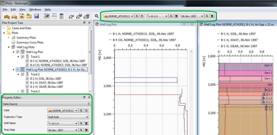
It is possible to change some data source parameters in one go for either a full plot or several selected curves. To change the parameters for a whole plot use either the Data Source group in the Property Editor for the Well Log Plot or corresponding toolbar which is visible when a Well Log Plot or any of its children are selected. Changing parameters in the Data Source group for the plot will also change the source for Zonation/Formations and Well Path Attributes in addition to the data source for all Well Log Extraction Curves and Well Log LAS Curves.
The source stepping icons
 allows to quickly step through cases, wells, and timesteps c.f.
Summary Plot Source Stepping.
allows to quickly step through cases, wells, and timesteps c.f.
Summary Plot Source Stepping.
To change data source for curves, select the curves for which you wish to change source and select Change Data Source from the right-click menu. The following dialog will appear:
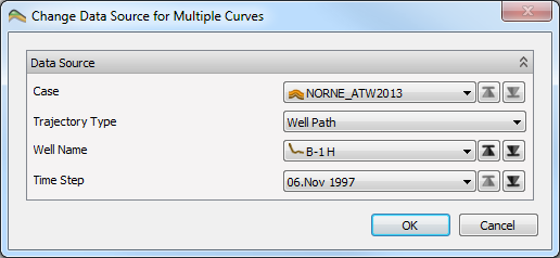
In both cases, the following parameters are available to change:
- Case – Applies the selected case to all the curves.
- Trajectory Type – Sets whether to use Simulation Wells or Well Paths as a data source for all curves.
- Well Name – Applies this well path to all the curves.
- Time Step – Applies this time step to all the curves.
Common for the different ways of changing data source is that if a parameter is not shared among all the curves, the drop down list will show “Mixed Cases, “Mixed Trajectory Types”, “Mixed Well Paths” or “Mixed Time Steps” to indicate that the curves have different values for that parameter. It is still possible to select a common parameter for them which will then be applied across the curves.
Well Log RFT Curves
Well Log RFT Curves shows the values in a RFT file. See RFT Plot for details about RFT. A curve in a RFT plot will look identical to a RFT curve in a well log plot, if the depth type of the well log plot is TVD, and the interpolation type of the curve is Point to Point.
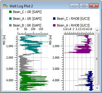
Well Log LAS Curves
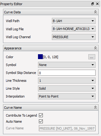
LAS-curves shows the values in a particular channel in a LAS-file.
The property panel of a LAS-curve is shown below:
Note
You can also create a LAS-curve by a simple drag-drop operation in the Project Tree: Drag one of the LAS channels and drop it onto a Track. A new curve will be created with the correct setting.
LAS-file Support
Importing LAS-files
See Importing Well Log Files for details on LAS file import.
Exporting LAS-files
A set of curves can be exported to LAS files by right-clicking the curves, well log track, or well log plots in Plot Project Tree and select Export To LAS Files …. An export dialog is displayed, allowing the user to configure how to export curve data.
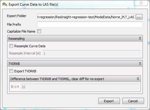
- Export Folder – Location of the exported LAS files, one file per unique triplet of well path, case and time step.
- Resampling – If enabled, all curves are resampled at the given resample interval before export.
- TVDRKB – If enabled, TVDRKB for all curves based on the listed well paths are exported. If the difference field is blank, no TVDRKB values are exported.