Well Bore Stability Plots
ResInsight can create Well Bore Stability plots for Geomechanical cases. These plots are specialized Well Log Plots to visualize Formations, Well Measurements, Well Path Attributes as well as a set of well path derived curves in different tracks.
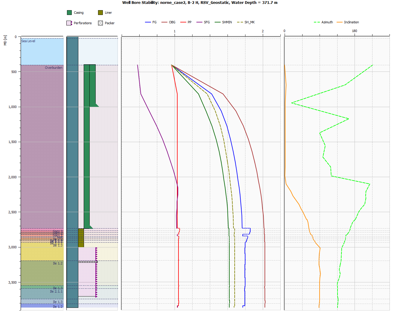
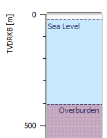
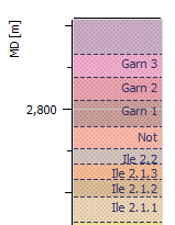
In the figure above, the first track contains Formations and an indication of sea level.
| Sea Level | Formations |
|---|---|
|
|
The second track contains a visualisation of the well, with well attributes of Casing Design as well Completions
The third track, which is disabled by default, contains the input parameters of the plot as described in the Input Requirements section.
The fourth track (third visible by default) shows the following stability gradients (all normalized by mud weight):
- FG: Fracture Gradient in sands based on Kirsch and in shale based on the K0_FG parameter or proportional to SHMIN.
- OBG: Overburden stress gradient: Stress component S_33.
- PP: Pore pressure.
- SFG: Shear Failure Gradient for shale based on Stassi-d’Alia.
- SHMIN: Minimum horizontal stress from grid.
- SH_MK: Minimum horizontal stress from Matthews & Kelly.
The fifth track contains curves showing the angular orientation of the well path as azimuth (deviation from vertical) and inclination (deviation from x-axis) in degrees.
If any Well Measurements are present, they will be visible as symbols in the track Stability Curves.
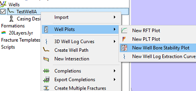
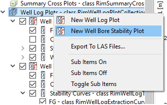
Create Well Bore Stability plots
Well Bore Stability plots can be created from the right-click menu for a well path in Project Tree or from the the right-click menu of the Well Log Plots entry in Plot Project Tree. In the former case, the well bore stability plot will be created for the selected Well Path. In the latter case, it will be created for the first well path in the well path list and the well path for the entire plot can be changed with the Change Data Source Feature.
Input requirements
In order to calculate PP, FG, SFG and SH_MK, the following input parameters are required:
| Curve | Required Parameters |
|---|---|
| PP | Pore Pressure in reservoir (PP Reservoir) and outside the reservoir (PP Non-Reservoir) |
| FG | Pore Pressure (PP Reservoir), Poissons’ Ratio in Sand, FG Shale in shale |
| SFG | Uniaxial Compressive Strength (UCS) |
| SH_MK | K0_SH, Overburden Gradient at initial time (OBG0) and the Depletion Factor (DF) |
For parameters with multiple available sources, the sources will be tried in numbered order for each curve point (where well path intersects with grid). However, the options for FG Shale are mutually exclusive and will apply to the whole domain.
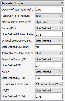
| Parameter | Default | Sources |
|---|---|---|
| Density of Sea Water | $1.03 g/cm^3$ | User setting in GUI |
| PP Reservoir | Grid Nodal Values (POR) | 1. Grid (Grid units), 2. LAS-file as equivalent mud-weight (Variable: “PP_INP” or “PP_RES_INP”, Units: SG_EMW), 3. Element Property Table (Variable: “POR_INP” with Units: Pascal or Variable: “PP_INP” with Units: SG_EMW) |
| PP Non-Reservoir | Hydrostatic PP (from TVDRKB, Density of Sea Water and gravity) | 1. LAS-file as equivalent mud-weight (Variable: “PP_NONRES_INP”, Units: SG_EMW), 3. Element Property Table (Variable: “POR_NONRES_INP” with Units: Pascal or Variable: “PP_NONRES_INP” with Units: SG_EMW), 4. Hydrostatic Pressure |
| Poissons’ Ratio | 0.35 | 1. LAS-file (Variable: “POISSON_RATIO_INP”), 2. Element Property Table (Variable: “POISSON_RATIO_INP”) |
| UCS | 100 bar | 1. LAS-file (Variable: “UCS_INP”, Units: bar), 2. Element Property Table (Variable: “UCS_INP”, Units: Pascal) |
| Initial Overburden Gradient (OBG0) | OBG at initial time step | 1. Grid (Grid units), 2. LAS-file (Variable: “OBG0_INP”, Units: Bar) |
| DF | 0.7 | 1. LAS-file (Variable: “DF_INP”, No Units), 2. Element Property Table (Variable: “DF_INP”, No units), 3 User Defined |
| K0_SH | 0.65 | 1. LAS-file (Variable: “K0_SH_INP”, No Units ), 2. Element Property Table(“Variable: “K0_SH_INP”, No Units), 3. User Defined |
| FG Shale | Derived from K0_FG | Derived from K0_FG and PP Non-Reservoir, Proportional to SH or LAS-file (Variable: “FG_SHALE_INP”, Units: SG_EMW) |
| K0_FG | 0.75 | 1. LAS-file (Variable: “K0_FG_INP”, No Units ), 2. Element Property Table(“Variable: “K0_FG_INP”, No Units), 3. User Defined |
In addition to the units above, it LAS-files it is possible to supply PP in Bar and UCS in Pascal or MPa. Conversion will be handled automatically.
Equations and calculations
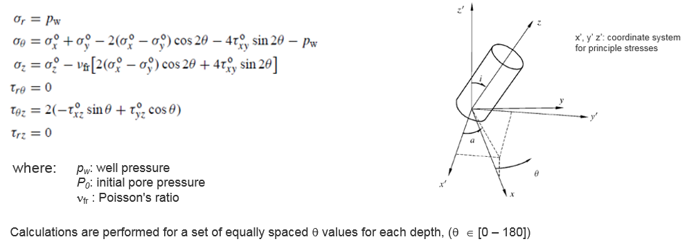
Stresses at the borehole wall - Kirsch equations
The basic input to wellbore stability models is the stresses at the borehole wall given by the Kirsch equations in cylindrical coordinates:
The transformation of stresses from cartesian coordinate system to x’, y’, z’ is performed by pre- and transposed postmultiplication of the stress tensor with a 3x3 transformation matrix M, i.e.
![]() .
.
Fracture gradient calculations based on Kirsch in sand
To estimate the fracture gradient FG, first step is to find the principal effective stresses at the borehole wall:
$$\sigma’_1 = \sigma’_1 (\theta)= \sigma’_r = p_w - p_0$$
$$\sigma’_2 = \sigma’_2 (\theta) = \sigma_{t \max} = \frac{1}{2} \left( (\sigma_z + \sigma_\theta) + \sqrt{(\sigma_z - \sigma_\theta)^2 + 4\tau_{\theta z}^2} \right) - p_0$$
$$\sigma’_2 = \sigma’_3 (\theta) = \sigma_{t \min} = \frac{1}{2} \left( (\sigma_z + \sigma_\theta) - \sqrt{(\sigma_z - \sigma_\theta)^2 + 4\tau_{\theta z}^2} \right) - p_0$$
Next step is to solve for the value of $\theta \in [0 - 180]$ that yields $\sigma’_3 (\theta) = 0$ which in turn gives us $\sigma_\theta$ which can be used to solve for $P_w$ in the Kirsch equations.
Then calculate FG in equivalent mud weight units as $$ FG = \frac{P_w}{TVD_{RKB} \: g \: \rho}$$ where $TVD_{RKB} = TVD_{MSL} + AirGap$, the gravity acceleration $g = 9.81 m/s^2$ and the density of sea water $\rho$ in $kg/m^3$ (thus 1000 x the UI input in $g/cm^3$).
Fracture gradient in shale
$$FG_{shale} = K0_{FG} \times (OBG0 - PP0) + PP0$$
SH from Matthews & Kelly
$$SH_{MK} = K0_{SH} \times (OBG0 - PP0) + PP0 + DF \times (PP-PP0)$$
Stassi-d’Alia failure criterion in shale
Stassi-d’Alia failure criterion in shale is calculated by finding the well pressure $P_w$ that satisfies the following equation for $\theta \in [0 - 180]$:

where
 are the effective principal stresses from the Fracture Gradient calculation.
and UCS is the uniaxial compressive strength.
are the effective principal stresses from the Fracture Gradient calculation.
and UCS is the uniaxial compressive strength.
The Shear Failure Gradient is then given as
$$SFG = \frac{P_w}{TVD_{RKB} \: g \: \rho}$$
Python Interface
The ResInsight Python API offers functionality for creating Well Bore Stability Plots from Python. For an example of use, see ResInsight Python API, and the Create WBS Plot script listed under Python Examples.