Decline Curve Analysis
Create Decline Curves
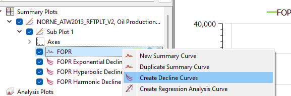
Decline Curve Analysis (DCA) can be created from the right-click menu for a curve in the Plot Project Tree.
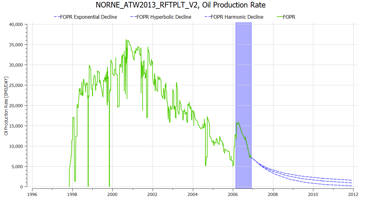
Three decline curves are created, and the values for the decline curves can be inspected visually in the plot and values can be displayed using Show Plot Data from the menu inside the plot window.
Origins
J.J. Arps [1] concluded that the decline in oil production rate ($q_i$) over time can be described by these equations:
$$\frac{ 1 }{ q_0 } \frac{\partial q_0}{ \partial t} = -D$$
where the decline rate, $D$ is a time-dependent function:
$$D = \frac{D_i}{1+bD_i t}$$
where:
- $q_0$ is the production rate (e.g. oil production) in a unit of choice (e.g STB/day)
- $t$ is the time
- $D$ is the time dependent decline rate
- $D_i$ is the initial decline rate (constant)
- $b$ is a dimensionless constant (typically used as a tuning parameter to match actual field data) and is in the range of $ 0 <= b <= 1 $.
The equations can be used to forecast future reservoir and well production.
Based on the value of $b$ in the function, Arps classified the decline curves into three types:
- The exponential decline has $b = 0$.
- The harmonic decline has $b = 1$.
- The hyperbolic decline has $b$ ranges between 0 and 1.
It is important to note that the decline curve is an empirical model and assumes a simplified representation of the complex physical and geological factors affecting production decline.
Rate-Time Decline Curves
Exponential Decline
Exponential decline is the production decline when $ b = 0 $. This gives a constant decline ($D_i = D$).
$$q_0 = q_i e^{-Dt }$$
Hyperbolic Decline
Hyperbolic decline is the generic case where $ 0 < b < 1 $.
$$q_0 = \frac{q_i}{ (1+bD_i t )^\frac{1}{b} }$$
Harmonic Decline
Harmonic decline is the production decline when $b = 1$:
$$q_0 = \frac{q_i}{ (1+D_i t ) }$$
Rate-Cumulative Production Decline Curves
Exponential Decline
Exponential decline is the production decline when $b = 0$. This gives a constant decline ($D_i = D$).
$$N_p = \frac{q_i - q_0}{D}$$
Hyperbolic Decline
Hyperbolic decline is the generic case where $ 0 < b < 1 $.
$$N_p = \frac{q_i^b}{D_i(1-b)} [q_i^{(1-b)} - q_0^{(1-b)}]$$
Harmonic Decline
Harmonic decline is the production decline when $ b = 1 $:
$$N_p = \frac{q_i}{ D_i } * \ln(\frac{q_i}{ q_0} )$$
Decline Rate
The continuous decline rate ($D_i$) can be determined from production history data. Using production rate and time data the value is the slope of the straight line on a semi-log plot. Taking two points on from the data $(t_1, q_1)$ and $(t_2, q_2)$:
$$D_i = \frac{1}{t_2 - t_1} \ln(\frac{q_1}{q_2})$$
where:
- $t_1$ is the time of the first point.
- $q_1$ is the production rate in the first point.
- $t_2$ is the time of the second point.
- $q_2$ is the production rate in the second point.
References
[1] Arps, J. J.: “Analysis of Decline Curves,” SPE-945228-G, Trans. of the AIME (1945)