Flow Diagnostics Plots
Flow Diagnostics Plots can be used to view well allocation, well inflow rates, cumulative saturation along time of flight and flow characteristics.
They are managed from the folder Flow Diagnostics Plots located in Plot Project Tree in the Plot Main Window.
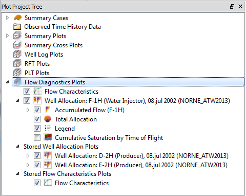
This folder contains a default Flow Characteristics Plot and Well Allocation Plot. In addition, two folders with stored well allocation and flow characteristics plots will show up if there are any of those in the model.
Please refer to Cell Results-> Flow Diagnostic Results for a description of the results and references to more information about the methodology.
Well Allocation Plots
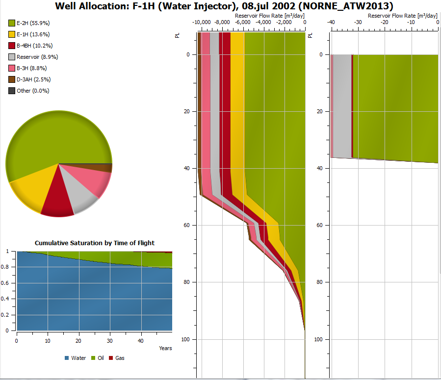
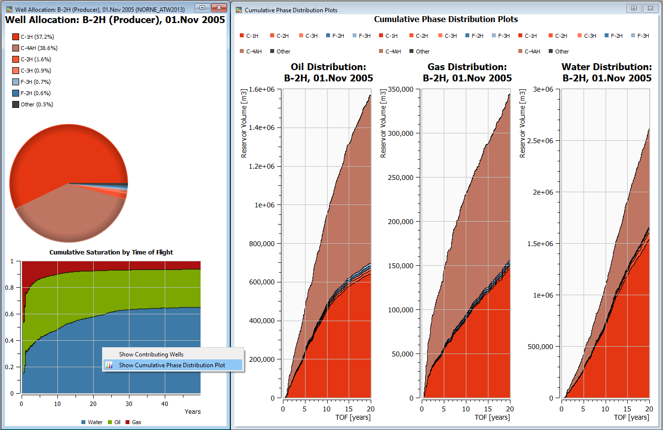
Well allocation plots show the flow along a specified well, along with either phase distribution or the amount of support from/to other wells. The total phase or allocation is shown in the legend and as a pie chart, while the well flow is shown in a depth value vs flow graph.
In addition a Cumulative Saturation by Time of Flight plot may be shown. This little plot illustrates how the total saturation changes as you go from the well-connection-cells along increasing time of flight adding the cells as you go.
Branches
Each branch of the well will be assigned a separate Track. For normal wells this is based on the branch detection algorithm used for Well Pipe visualization, and will correspond to the pipe visualization with Branch Detection On ( See Well Pipe Geometry ). Multi Segment Wells will be displayed according to their branch information, but tiny branches consisting of only one connection are lumped into the main branch to make the visualization more understandable ( See Dummy branches ).
Creating Well Allocation Plots
To plot the Well allocation for a well, right-click the well in the Project Tree or in the 3D View and invoke the command Plot Well Allocation.
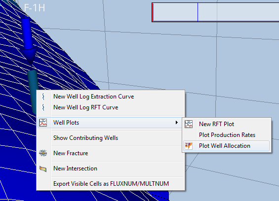
The command updates the default Well Allocation Plot with new values based on the selection and the settings in the active view. This plot can then be copied to the Stored Plots folder by the right-click command Add Stored Well Allocation Plot.
Options
The Legend, Total Allocation pie chart, Cumulative Saturation, and the Well Flow/Allocation can be turned on or off from the toggles in the Project Tree. The other options are controlled from the property panel of a Well Allocation Plot:
- Name – Auto generated name used as plot title
- Show Plot Title – Toggles whether to show the title in the plot
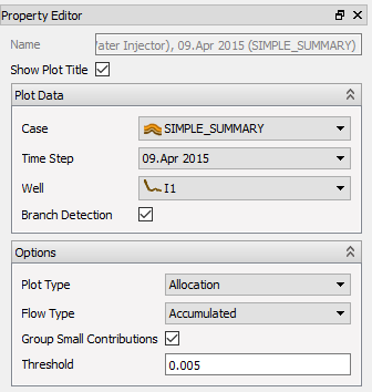
- Plot Data – Options controlling when and what the plot is based on
- Case – The case to plot data from
- Time Step – The selected time step
- Well – The simulation well to plot
- Options
- Plot Type
- Allocation – Plots Reservoir well flow rates along with how this well supports/are supported by other wells ( This option is only available for cases with Flux results available )
- Well Flow – Plots Surface Well Flow Rates together with phase split between Oil, Gas, and Water
- Flow Type
- Accumulated – Plots an approximation of the accumulated flow along the well
- Inflow Rates – Plots the rate of flow from the connection into the well
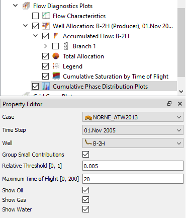
- Group Small Contributions – Groups small well contributions into a group called Other
- Threshold – Threshold used by the Group Small Contributions option
- Plot Type
Depth Settings
The depth value in the plot can be controlled by selecting the Accumulated Flow/Inflow Rates item in the Project Tree. This item represents the Well-Log-like part of the Well Allocation Plot and its properties are shown below:
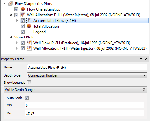
- Name – The plot name, updated automatically based on the Flow Type and well.
- Depth Type
- Pseudo Length – Use the length along the visualized simulation well pipe as depth.
In this mode the curves are extended somewhat above zero depth keeping the curve
values constant. This is done to make it easier to see the final values of the curves relative to each other.
The depth are calculated with Branch detection On and using the Interpolated well pipe geometry.
( See Well Pipe Geometry ) - TVD – Use True Vertical Depth on the depth-axis. This will produce distorted plots for horizontal or near horizontal wells.
- Connection Number – Use the number of connections counted from the top on the depth-axis.
- Pseudo Length – Use the length along the visualized simulation well pipe as depth.
In this mode the curves are extended somewhat above zero depth keeping the curve
values constant. This is done to make it easier to see the final values of the curves relative to each other.
- Visible Depth Range – These options control the depth zoom.
- Auto Scale – Toggles autoscale on/off. The plot is autoscaled when significant changes to its settings are made.
- Min, Max – Sets the visible depth range. These are updated when zooming using the mouse wheel etc.
Accessing the Plot Data
The command right-click command Show Plot Data will show a window containing the plot data in ascii format. The content of this window is easy to copy and paste into Excel or other tools for further processing.
It is also possible to save the ascii data to a file directly by using the right-click command Export Plot Data to Text File on the Accumulated Flow/Inflow Rates item in the Project Tree.
The total accumulation data can also be viewed in ascci format by the command Show Total Allocation Data.
Producer/Injector Connectivity Table
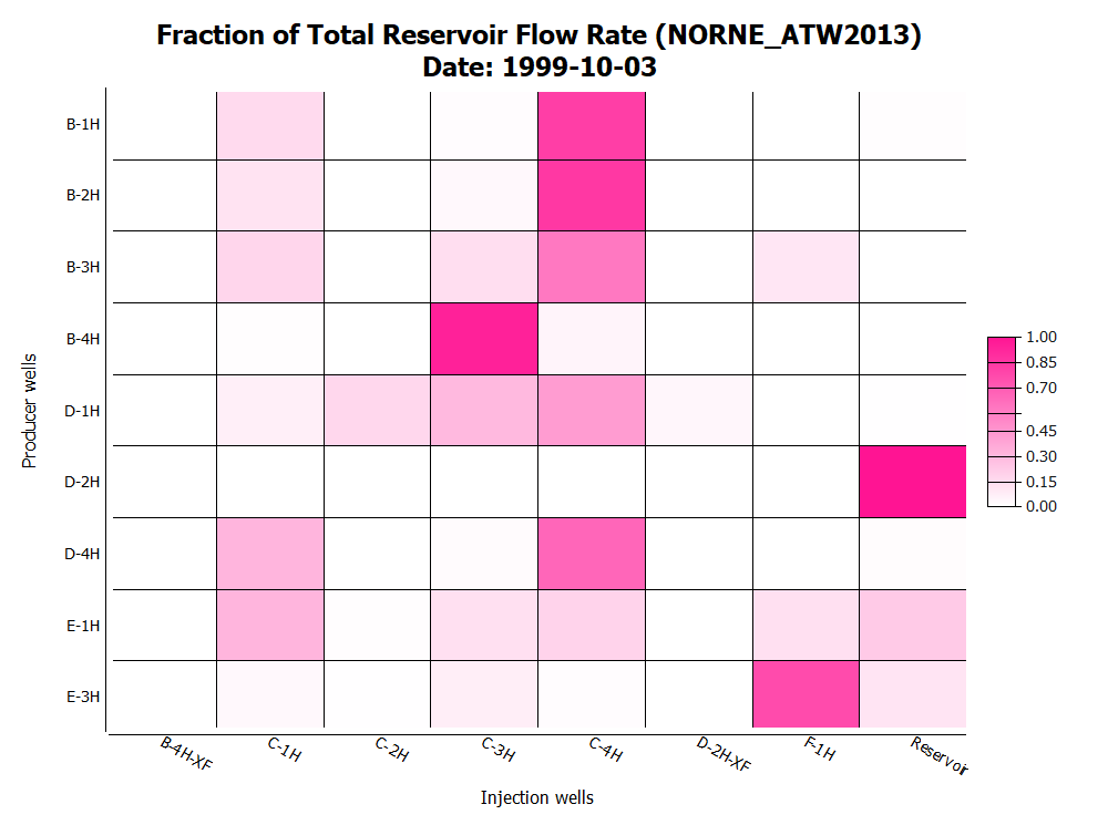
Use Producer/Injector Connectivity Table to see the flow diagnostics communication between producer and injector wells for selected time steps.
Well Allocation Over Time
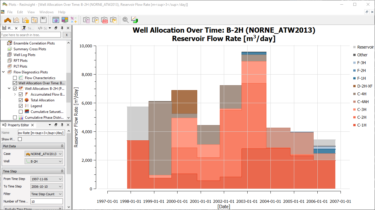
Use Well Allocation Over Time to see the allocation over multiple restart time steps.
Cumulative Phase Distribution Plot
A Cumulative Phase Distribution Plot shows the volumetric oil, gas, and water distribution from contributing wells to a target well. For producer B-2H, for instance, such a plot can be created by right-clicking its entry under Simulation Wells in Project Tree.
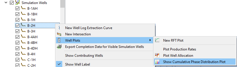
A Cumulative Phase Distribution Plot can also be created by right-clicking a Cumulative Saturation plot, c.f. figure below.
Clicking its entry in Plot Project Tree, displays content and settings of the Cumulative Phase Distribution Plot.
Flow Characteristics Plot
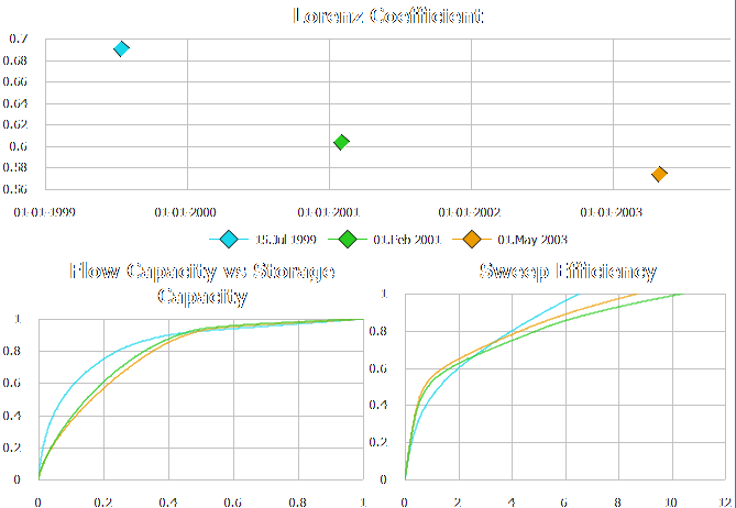
This window displays three different graphs describing the overall behavior of the reservoir for each time step from a flow diagnostics point of view.
- Lorenz Coefficient – This plot displays the Lorenz coefficient for the complete reservoir for each selected time step. The time step color is used as a reference for the time step in the other graphs.
- Flow Capacity vs Storage Capacity – This plot displays one curve for each time step of the F-phi curve for the reservoir.
- Sweep Efficiency – This plot displays one Sweep Efficiency curve for each selected time step.
Settings
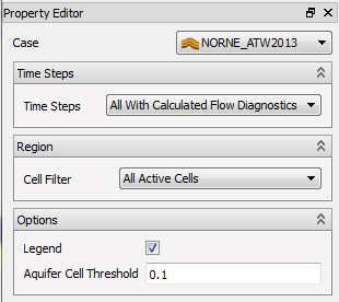
- Case – Selects the source case for the plot.
- Time Steps – These options selects the time steps to be used in the plot.
- All With Calculated FlowDiagnostics – Plot data from all the time steps already solved by the Flow Diagnostics Solver, but nothing more. The solver will be run implicitly when the user requests any Flow Diagnostics results on a particular time step using Cell Results, Well Allocation Plots, or Well Log Extraction Curves.
- Selected – Use the selected time steps only. Activating this options displays a listbox with all the available time steps in the 3D case. Time steps already solved by the Flow Diagnostics Solver are marked with an asterix
*. Select the interesting time steps and press apply to invoke the solver for unsolved time steps, and to show them in the plot.
- Region – These group of options controls the cell region of interest for the plot.
- Cell Filter – Selects the type of cell filtering to apply. Sub-options are displayed depending on the selection.
- All Active Cells – Use all the active cells in the model (default)
- Visible Cells – Use the visible cells in a particular predefined view as cell region. This option will respect all the filter settings in the view, and use the correct cell set for each time step.
- View – The view to use as cell filter
- Injector Producer Communication – The region of communication between selected producers and injectors. See Flow Diagnostic Results
- Tracer Filter – Wild card based filter-text to filter the list of tracers
- list – Producer and injector tracers to select
- Show Region – Button to create (or edit) a 3D View showing the selected region of cells.
- Min communication – A threshold for the cells communication value. Cells with communication below this threshold is omitted from the region.
- Flooded by Injector/Drained by Producer – The region with a Time Of Flight from the selected tracers below the selected threshold.
- Tracer Filter/list/Show Region – See above.
- Max Time of Flight [days] – Only cells with a Time of Flight value less then this value are used.
- Cell Filter – Selects the type of cell filtering to apply. Sub-options are displayed depending on the selection.
- Options
- Legend – Toggles the legend on/off
- Aquifer Cell Threshold – This threshold can be used to exclude unwanted effects of aquifers. Cells are excluded if their pore volume are larger than threshold
*total pore volume.